Frustrated Magnetism
When you add competing interactions to the Ising model, spins can't satisfy all their neighbors at once. This is frustration — and the \(J_1\)-\(J_2\) model on the square lattice is its textbook Ising example. This page reproduces its two ordered phases and the phase diagram between them; the model is the one studied in the research that mcising was written for (Çivitcioğlu, Römer & Honecker, Phys. Rev. E 111, 024131 (2025)).
mcising's Hamiltonian is
so a positive coupling favors aligned pairs and a negative one favors anti-aligned pairs.
J1-only: the clean case
With only nearest-neighbor coupling, the ground state is simple — all spins align:
from mcising import Simulation, SimulationConfig, LatticeConfig

config = SimulationConfig(
    lattice=LatticeConfig(size=32, j1=1.0),
    temperatures=(3.0, 2.269, 1.5),
    n_sweeps=1000,
    seed=42,
)

results = Simulation(config).run()
Competing J2 < 0: the stripe phase
\(J_2\) couples the four diagonal neighbors of every site. With \(J_1 > 0\) and \(J_2 < 0\) the two couplings compete: \(J_1\) wants every nearest-neighbor pair aligned, which automatically aligns the diagonals as well — exactly what a negative \(J_2\) penalizes. Two candidate ground states result (energies per site on a periodic lattice):
| State | Pattern | Energy per site |
|---|---|---|
| Ferromagnet | all spins up | \(e_\mathrm{FM} = -2J_1 - 2J_2\) |
| Stripe (superantiferromagnet) | rows (or columns) alternate | \(e_\mathrm{stripe} = 2J_2\) |
In the stripe state every site has two aligned and two anti-aligned nearest neighbors, so the \(J_1\) bonds cancel, while all four diagonal bonds are anti-aligned and satisfy \(J_2 < 0\). The two energies cross at \(J_2 = -J_1/2\): for \(-1/2 < J_2/J_1 < 0\) the ground state is ferromagnetic, for \(J_2/J_1 < -1/2\) it is the stripe. The stripe breaks the lattice's rotation symmetry, so its order parameter is the staggered magnetization along one axis,
which is not a built-in observable — but the stored configurations make it a few lines of NumPy. Cool the lattice through the transition at \(J_2 = -0.6\) and watch \(\langle |m| \rangle\) stay near zero while \(m_s\) saturates:
import numpy as np
from mcising import Simulation, SimulationConfig, LatticeConfig


def stripe_order(configurations: np.ndarray) -> np.ndarray:
    """Per-snapshot stripe order parameter of (n, L, L) configurations."""
    n, rows, cols = configurations.shape
    spins = configurations.astype(float)
    along_rows = np.abs((spins * (-1.0) ** np.arange(rows)[None, :, None]).mean(axis=(1, 2)))
    along_cols = np.abs((spins * (-1.0) ** np.arange(cols)[None, None, :]).mean(axis=(1, 2)))
    return np.maximum(along_rows, along_cols)


config = SimulationConfig(
    lattice=LatticeConfig(size=16, j1=1.0, j2=-0.6),
    temperatures=(3.0, 2.0, 1.2, 0.6),  # descending: a cool-down ladder
    n_sweeps=400,
    n_thermalization=200,
    seed=42,
)
results = Simulation(config).run(show_progress=False)

for T in results.temperatures:
    m = np.abs(results.magnetization[T]).mean()
    m_s = stripe_order(results.configurations[T]).mean()
    print(f"T={T:.1f}: <|m|>={m:.3f}  <m_s>={m_s:.3f}")
Metropolis only, and cool down — don't quench
Wolff and Swendsen-Wang are only correct for a single ferromagnetic coupling; SimulationConfig refuses them when \(J_2 \neq 0\), so frustrated runs use Metropolis. Give it a descending temperature ladder (the default cool-down mode carries the final state of each temperature into the next). A single low temperature from a random start is a quench that freezes into domain walls, and near \(J_2 = -J_1/2\), where the two ground states are almost degenerate, Metropolis equilibrates slowly at low \(T\) — that is the regime for parallel tempering.
The phase diagram
Scanning \(J_2\) from \(-1\) to \(0\) with a cool-down ladder at every value maps both order parameters over the \((J_2, T)\) plane. The committed script examples/stripe_phase_diagram.py produces this figure in under a minute; the specific-heat peak at each \(J_2\) (white line) is a finite-size estimate of the transition temperature, which falls towards zero from both sides of \(J_2 = -J_1/2\) (dotted):
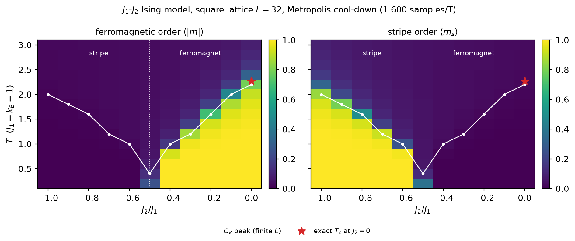
The transition out of the stripe phase is weakly first order for \(1/2 < |J_2|/J_1 \lesssim 0.67\) and continuous with continuously varying, Ashkin-Teller-like exponents beyond that — see Kalz, Honecker & Moliner, Phys. Rev. B 84, 174407 (2011) and Jin, Sen & Sandvik, Phys. Rev. Lett. 108, 045702 (2012). Resolving that requires finite-size scaling across several \(L\), which the example script leaves to you (it is a map at one \(L\), not a scaling study).
What the sign of J2 does
Positive \(J_2\) favors aligned diagonal neighbors and simply reinforces \(J_1\) — the ferromagnet survives with a higher \(T_c\). Negative \(J_2\) competes with \(J_1\); the ratio \(J_2/J_1\) controls the degree of frustration and \(J_2/J_1 = -1/2\) is the maximally frustrated point.
J1-J2-J3: the full Hamiltonian
Add third-nearest-neighbor coupling for even richer phase behavior:
config = SimulationConfig(
    lattice=LatticeConfig(size=32, j1=1.0, j2=-0.6, j3=0.3),
    temperatures=(3.0, 2.269, 1.5),
    n_sweeps=1000,
    seed=42,
)

results = Simulation(config).run()
mcising automatically selects the optimal Metropolis strategy from 15 pre-built lookup tables based on which couplings are active. No performance cost for adding J2 or J3.
External magnetic field
Break the up/down symmetry with an external field h:
config = SimulationConfig(
    lattice=LatticeConfig(size=32, j1=1.0, h=0.5),
    temperatures=(3.0, 2.269, 1.5),
    n_sweeps=1000,
    seed=42,
)

results = Simulation(config).run()
With h > 0, the system prefers spin-up even above Tc. The phase transition becomes a crossover instead of a sharp transition.
Frustration on different lattices
Different lattice geometries give different frustration physics:
from mcising import LatticeType

config = SimulationConfig(
    lattice=LatticeConfig(
        lattice_type=LatticeType.TRIANGULAR,
        size=32, j1=-1.0,
    ),
    temperatures=(4.0, 2.0, 1.0),
    n_sweeps=1000,
)
The triangular lattice with antiferromagnetic \(J_1\) is geometrically frustrated without any \(J_2\): no configuration satisfies all three bonds of a triangle, the ground state is macroscopically degenerate, and the model has no ordered phase at any \(T > 0\) (Wannier 1950). Its ground-state energy per site is \(-|J_1|\), which the test suite checks exactly.
Tip
For frustrated systems near critical points, consider using Parallel Tempering — replica swaps help escape local energy minima that trap standard Metropolis.